
This manual is also available as PDF document.
Sometimes you can't get outdoors. Now and then there are rainy days. That's when you could combine one with the other. A quick project for indoors and the use of the same outdoors is ideal.
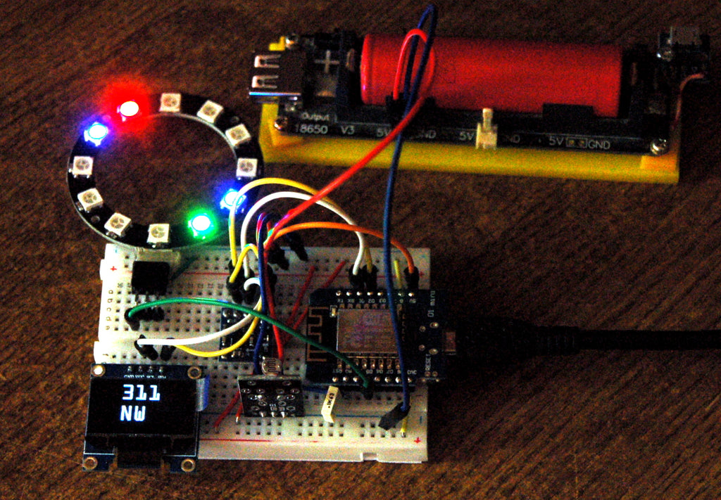
Image 1: Compass in action
Almost exactly a year ago, I had a look at the SIM800 GPS module. There are a number of blog posts about it, for example this one. At that time I already planned to add a compass application to the system. Exactly that is to be done now with this contribution. What risks and side effects occurred, I tell you in the current episode from the series
MicroPython on the ESP32 and ESP8266
today
The ESP8266 compass
Besides an ESP8266 D1 Mini, which I chose because of its small dimensions, the magnetometer module GY-271 with a DE5883L as the most important component, an OLED display, an LDR module and a neopixel ring are used. A battery unit with three AA cells, or better a battery holder with a 16850 Li-battery can serve as a power supply in case of need.
This brings us to the list of the necessary hardware.
Hardware
|
1 |
D1 Mini NodeMcu with ESP8266-12F WLAN module or |
|
1 |
LED Ring 5V RGB WS2812B 12-Bit 37mm or similar |
|
1 |
|
|
1 |
|
|
1 |
|
|
1 |
|
|
1 |
|
|
various |
|
|
1 |
Breadboard Kit - 3 x 65pcs Jumper Wire Cable M2M and 3 x Mini Breadboard 400 Pins |
|
optional |
The ESP8266s have an unpleasant characteristic, which can be turned off with certain measures - they all restart sporadically for seemingly invisible reasons. There are at least two reasons for this. The hardware-related reason is a certain sensitivity to too low and/or unclean operating voltage. Voltage fluctuations on the USB bus can already be enough for the little one to reboot in an irregular rhythm of a few seconds. A separate power supply or a battery box with at least three, better 4 AA cells can help. Such reboots are probably caused by the AP interface, which is booted by the firmware with every reboot, no matter if it is needed or not. Due to the higher current consumption when the AP interface is activated, the voltage briefly collapses and triggers a restart. If the interface is switched off, peace returns.
>>> import network; network.WLAN(network.AP_IF).active(False)
A capacitor of 0.1µF from the EN pin to GND and a pullup resistor of 4.7KΩ against Vcc=3.3V sometimes already work wonders, as well as an electrolytic capacitor of 100µF at the supply voltage.
The neopixel ring serves as an indicator of the north-south direction even in darkness. The brightness of the LEDs is adjusted to the ambient brightness by the LDR (Light-Dependent-Resistor = photoresistor). On the OLED display, you can read the bearing angle to the nearest degree and the cardinal direction in a 22.5-degree grid.
The magnetic sensor is a DE5883L = QMC5883L, which should not be confused with the HMC5883L. Besides different physical properties, the DE5883L has a completely different register arrangement than the HMC5883L. Also, the hardware addresses of the devices are different, for the QMC5883L it is the 7-bit address 0x0D. For use as a compass, it is essential to calibrate the sensor to bring the sensitivity of the x- and y-axis to the same level and the same zero line. Only then a conversion of the magnetic data into angles is possible.
The circuit is shown in figure 2. The button at D3=GPIO0 can be pressed at startup to initiate a new calibration of the QMC5883L.

Image 2: Compass - circuit
This brings us to the software for the project.
The software
For flashing and programming the ESP32:
Thonny or
Used firmware for the ESP8266/ESP32:
Please choose a stable version
ESP8266 with 1MB Version 1.18 Status: 25.03.2022 or later
The MicroPython programs for the project:
ssd1306.py: Display driver for the OLED module
oled.py: normal display driver for the OLED module
micropython-font-to-py: package by Peter Hinch for cloning Windows fonts. Included is writer.py, the driver for the generated fonts. From this file, I removed the not needed parts, so that everything fits into the ESP8266. Therefore you should better use the following file.
writer.py: stripped down the driver for the MicroPython character sets
ocr20.py: a character set with 20-pixel character height
Datasheet of the QMC5883L
test_calibration.py: Program to record the calibration curves
compass.py: Operating program to the compass.
MicroPython - Language - Modules and Programs
For the installation of Thonny, you will find here a detailed manual (english version). In it there is also a description of how the Micropython firmware (as of 05.02.2022) on the ESP chip burned is burned.
MicroPython is an interpreter language. The main difference to the Arduino IDE, where you always and only flash whole programs, is that you only have to flash the MicroPython firmware once at the beginning to the ESP32, so that the controller understands MicroPython instructions. You can use Thonny, µPyCraft or esptool.py to do this. For Thonny, I have described the process here described here.
Once the firmware is flashed, you can casually talk to your controller one-on-one, test individual commands, and immediately see the response without having to compile and transfer an entire program first. In fact, that's what bothers me about the Arduino IDE. You simply save an enormous amount of time if you can do simple tests of the syntax and the hardware up to trying out and refining functions and whole program parts via the command line in advance before you knit a program out of it. For this purpose, I also like to create small test programs from time to time. As a kind of macro they summarize recurring commands. From such program fragments sometimes whole applications are developed.
Autostart
If you want the program to start autonomously when the controller is switched on, copy the program text into a newly created blank file. Save this file as boot.py in the workspace and upload it to the ESP chip. The program will start automatically at the next reset or power-on.
Test programs
Manually, programs are started from the current editor window in the Thonny IDE via the F5 key. This is quicker than clicking on the Start button, or via the menu Run. Only the modules used in the program must be in the flash of the ESP32.
In between times Arduino IDE again?
If you want to use the controller together with the Arduino IDE again later, simply flash the program in the usual way. However, the ESP32/ESP8266 will then have forgotten that it ever spoke MicroPython. Conversely, any Espressif chip that contains a compiled program from the Arduino IDE or the AT firmware or LUA or ... can easily be flashed with the MicroPython firmware. The process is always here described.
Contacting (Micro)Python
If you have already worked with the Arduino IDE, you may have had the urge to try out a command now and then to investigate its behavior. But there an interactive work with the system is not provided, I have already mentioned this above.
MicroPython as a descendant of the interpreter language C-Python behaves differently. You work in an IDE, an integrated development environment, with a direct line to a Python interpreter. In Python, this tool is called REPL. This is an acronym for the states Read - Evaluate - Print - Loop. You make an input at the terminal, the MicroPython interpreter evaluates the input, returns a response, and waits for the next input. The Windows command prompt, formerly MS-DOS, works according to the same scheme.
There are quite a few IDEs, Thonny, µPyCraft are two of them, Idle and MU are two others. I like to work with Thonny because besides the terminal (REPL) and a comfortable editor for creating and testing programs, it also has 12 wizards, a plotter, and a tool for flashing the firmware. With REPL it is easy to test each instruction individually. We will try this out at various points in this manual. Inputs at the REPL prompt >>> I format as follows bold, the Answers from the system italic.
Another thing is different with Python than with C or other compiler languages. There is no type specification when declaring variables or functions. MicroPython figures out the type itself.
Some info about the I2C bus
I2C, actually I²C, meaning "I squared C" comes from IIC and that is an acronym for Inter-Integrated-Circuit. This describes a bus with two lines, SDA and SCL, which was developed by Philips to allow communication of units in a device. This is exactly the purpose for which we will use this bus connection today. The ESP8266 should be able to talk to the OLED display and the magnetometer module. The circuit conditions for operation are already fulfilled by the display and the GY271 module. It is about one pullup resistor each, which pulls the SCL and the SDA line against Vcc=3.3V. The HIGH level is also the idle state.
Each unit on the bus can pull the level of the line to GND potential through its output stage. The different states on the lines and their timing can be used to compose signals that are important for controlling the transmission: ST = start-condition (transmission start), SP = stop-condition (transmission end), ACK = acknowledge (data accepted) and NACK = not acknowledge, (data rejected, error condition).
The boss in our project is of course the ESP8266. As master, it specifies the clock of the transmission, 400.000Hz = 400 kHz. So in 2.5 µs one bit is transmitted. Normally, with a falling edge on the clock line SCL (serial clock) the data bit, 0 or 1, is switched to the data line SDA (serial data), LOW or HIGH, 0V or 3.3V. At the time of the rising edge on SCL, the state on SDA is read in as a data bit by the receiver. With the help of a logic analyzer you can make the signals visible. This can be enormously helpful in troubleshooting. By the way, you can find a description of the device in the blog post " Logic Analyzer - Part 1: Making I2C signals visible"by Bernd Albrecht. There it is also described how to sample the I2C bus. The little thing is connected to the USB bus and shows by means of a free software what is going on on the bus lines. Where the shape of pulses is not important, but only their timing, an LA is worth its weight in gold. And, while a DSO (digital storage oscilloscope) only provides snapshots of the waveform, with the LA you can sample over time and then zoom in on the interesting parts. This is shown in Figure 3 for the first part of the QMC5883L initialization sequence. The transmission starts with the start-condition - SDA is pulled LOW by the master while SCL is HIGH. The first byte to be output is the hardware address of the peripheral device, which is the 7-bit value 0x0D. The additional LSB (W) is 0 in this case because it is a subsequent write command. With a read access the 8th bit of the hardware address would be a 1. Each bit is marked by a dot.
The 9th bit is the ACK bit, which the QMC5883L uses to indicate that it has recognized the address. Therefore the QMC5883L now pulls the data line briefly to 0. In case of a NACK SDA would remain at 1. The hardware address is followed by the number of the register to be written, 0x09. Directly afterwards the data byte is transferred, 0x0D. A stop condition completes the transfer.

Image 3: Initialization of the QMC5883L (detail)
If the circuit is already built, we can run the first test.
>>> from machine import Pin, SoftI2C
>>> SCL=Pin(5)
>>> SDA=Pin(4)
>>> i2c=SoftI2C(SCL,SDA,freq=400000)
>>> i2c.scan()
[13, 60]
The scan command tells us that there are two I2C devices on the bus. We already know the address 13=0x0D, it belongs to the QMC5883L. The second address 60=0x3C addresses the OLED display.
In MicroPython the testing is done directly via REPL. In the Arduino IDE I would have to write the few lines into a program, compile it long and wide and send it as complete firmware to the ESP8266 to finally get the same information. Time to benefit, at least 100 : 1, with MicroPython I have 1:1 with immediate effect.
The magnetometer - QMC5883L
Before we get to the discussion of the program, a few notes about the magnetometer module. As mentioned above, there are two similar ICs, but they have completely different register numbers and also different technical characteristics. From the data sheet from qst I took the information for my class QMC5883L. This also fits to the chip DB5883L which is installed on the module GY-271.
The module has its own 3.3V regulator and also a level converter for the SCL and the SDA line. Also the necessary pullup resistors are already included. Thus the module can be connected to 5V operating voltage and can be connected to the ESP8266 without level problems.
The number of registers is manageable. Here the table 13 from page 16 of the datasheet.

Image 4: Register overview of the QMC5883L
The data registers for the three spatial axes are at the top of the list for the QMC5883L. The magnetometer data are stored as signed 16-bit values. Accordingly they are to be read in and processed. We actually only need the x- and y-direction. The method readAxes() from the class QMC5883L reads all axis registers anyway, because the datasheet says so. I will come to this later.
Two more data registers allow to read the temperature of the chip and with appropriate circulation also of the environment. According to the data sheet, chapter 9.2.3, page 17, the relative accuracy is specified with 100LSB/°C, which corresponds to an accuracy of 1/100°C. If the temperature indication shall correspond to the ambient values, then the zero point of the scale must be calibrated separately for each chip. The method readTemperature() demonstrates this. More about this later as well.
Register 0x06 can be understood as a status register. It reflects the state of the measuring unit. The bit DRDY interests us most in the context of the project, because it informs the ESP8266 that there is a new measured value. It is set by the QMC5883L when the data of all three axes have been transferred from the measuring unit to the I2C interface. It is cleared when all six axis registers have been read. So for this handshake to work, it is important to read all axis registers and test the DRDY bit before reading again. This is done by the method dataReady().
The bits OVL and DOR do not make a significant appearance in our project.
The registers 0x09 and 0x0A control the sequence of the measurements. The bits in the control register2 (0x0A) do not appear in the project. The Control Register1 is set to the value 0x0D during initialization. With an oversampling of 512 the noise behavior is reduced to a minimum. For the earth magnetic field 2G = 2 Gauss) are appropriate. Since 1970, the gauss is no longer a legal unit in the EU. It was replaced by the unit Tesla (T). 1 Gauss = 1G corresponds to the magnetic flux density of 100µT. The flux density in horizontal direction in Germany is about 20 µT, which corresponds to 0.2G. The yield of the sensor signal is therefore approx. 6400LSB of the sensor as a guide value.
The data output rate is set at 200 per second, and operation is continuous. An average of 100 individual measurements is taken to smooth the values, axesAverage().
So that everything works correctly afterwards, the register 0x0B must be written with a value of 0x01. Unfortunately, the data sheet does not give any further information about this.
At the first start of the program the sensor is calibrated. The OLED display informs that the calibration has been started and when it ends. During the process, the setup with the sensor must be rotated at least once in a horizontal position around the z-axis by at least 360 degrees. The program provides a duration of 20 seconds for this. Too fast rotation leads to inaccurate results. The calibration data are automatically saved to the file config.txt on the ESP8266 and read in during the next starts.
To check these values, a subsequent test can be performed using the angle network can be carried out. For this purpose, the angle net is first aligned exactly to the north using a normal magnetic compass and fixed on the table. There should be no iron parts in the immediate vicinity. also think of screws, nails, PC housings, etc. in, on and under the table.

Image 5: Aligning the measuring sheet
Now start the program once test_calbration.py from an editor window with F5.
>>> %Run -c $EDITOR_CONTENT
this is the constructor of OLED class
Size:128x64
QMC5883L is @ 13
This makes the methods of the QMC5883L class available on REPL and can be used to record the calibration table. We now create this table step by step with our test setup.

Image 6: Recording measurement curves
Just like the compass before, the breadboard is applied to the 0° line. The x-axis direction on the GY-271 module then also points in this direction. We call the method axesAverage(100) with the argument 100. We take 100 individual measurements, average the results and output the x and y values. We note these values to the angle 0°.
>>> k.axesAverage(100)
(1091, 68)
The process is repeated for each marker of the degree mesh. Finally, we enter all the values into a spreadsheet table. I did this in Libre Office and derived a graph from it. The calibration has gone well if the two curves have the same amplitude, are symmetrical about the right-hand axis, and, if possible, give a complete, smooth sin and cos curve. In Figure 7, therefore, the y-offset must be corrected somewhat.

Image 7: Calibration chart
Large TTF character sets for the OLED display
The calibration can be done well with the normal 8 pixel high standard font of the OLED display. But for the reading of the bearing angle and the rough celestial direction, a larger character set would be appropriate. And that is possible using the package micropython-font-to-py by Peter Hinch. With it you can clone TTF fonts from Windows into pixel-oriented fonts for MicroPython. Download the package from GitHub into a directory of your choice (here F:\font2py) and unpack it into a subdirectory, here f2p.
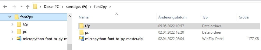
Figure 8: Installing the Font_to_py package
In the directory f2p I have a subdirectory sources (red dot) where I put the TTF fonts I want to convert. From the Windows fonts directory I copy the file OCRA.ttf to sources.

Image 9: Source directory for the selected fonts
With the Shift key held down (toggle uppercase) I right-click on f2p, select Open PowerShell window here in the context menu.

Image 10: Open PowerShell window in target directory
Now copy a font file from the Windows folder into the directory sources.

Image 11: TTF source files
For the further actions I use the font OCRA.ttf. Two steps represent the use of the font OCRA in size 20 pixels for use with our MicroPython program as module ocr20.py module. I create, to save memory only the really needed characters: 0123456789NWSO.

Image 12: Generating the required characters
The character information is now with all additional data in the file ocr20.pywhich must be copied to the workspace of the project. You can also see what the cloned character set looks like in the Powershell window.

Image 13: The OCRA20 character set for use in MicroPython
Besides the file ocr20.py for the representation of the large characters the modules ssd1306.py, oled.py and writer.py are needed. All four must be uploaded to the flash of the ESP8266.
The neopixel ring
A compass without a bearing aid is of little use. My bearing aid is a ring of 12 RGB LEDs of the type WS2812B, also known as Neopixel-LED. Each LED can be addressed via a common bus-like line (IN). Three bytes individually determine the brightness of the colors red, green and blue. A module in the standard firmware kernel enables simple setup and control.
The power supply is parallel. The data line leads serially from one LED unit to the next and represents a special kind of bus. Each unit contains an RGB LED and a controller that responds to the first incoming 24-bit sequence of color information. The signals, with the same period but different Duty Cycleare generated by a microcontroller, such as the ESP8266. 24 bits are generated per neopixel unit (8 each for green, red and blue). The period for one bit is 1.25µs +/-0.150µs, so the transmission frequency is about 800kHz. For a 1 the line is 0.8µs HIGH and 0.45µs LOW, a 0 is coded by 0.4µs HIGH and 0.85µs LOW. The first incoming 24 bits are processed by each WS2812B unit itself without passing them on. All now following bits are amplified and passed on to the next unit. The signal sequence from the microcontroller thus becomes 24 bits shorter from LED to LED. Unlike a usual data bus, the WS2812B units do not receive the data at the same time, but with a time delay of 24 bits times 1.25 µs/bit = 30 µs. This signal sequence is controlled in the ESP32/ESP8266 by MicroPython's built-in class machine.NeoPixel built in MicroPython. This makes the control of the LEDs very simple, which makes the application especially suitable for beginners.
A framebuffer (aka buffer) in the RAM memory of the ESP chip bins the color values (256 to the power of 3 = 16.7 million) between and the command NeoPixel.write() sends the information to the ring via the "bus" which is connected to a GPIO output (in our case GPIO14 = D5). That's all. Per color, red, green and blue, 256 brightness values can be set.
Several rings can be cascaded just like single LEDs by connecting the input of the next ring to the output of the previous one. The connections are made at the back, best by means of thin stranded wires.

Image 14: LED ring at the back - right feed, left forwarding
![]()
Image 15: Neopixel ring top side
The components for mixed colors are most easily determined experimentally via REPL. The brightness of the individual partial LEDs of a unit is quite different. So the RGB color codes in the tuples will rarely have the same value for the mixed colors.
>>> from neopixel import NeoPixel
>>> neoPin=Pin(14)
>>> neoCnt=12
>>> np=NeoPixel(neoPin,neoCnt)
>>> np[0]=(32,16,0)
>>> np.write()
For adjustment, the last two commands are repeated with different RGB code until the color reproduction matches. The values given here produce yellow as a mixed color of red and green. The output of the logic analyzer shows the coding of the individual bits. In addition, the plot reveals that the green value is transmitted before the red value. The yellow LED marks position 0 of the LED numbering on the ring.
![]()
Image 16: Neopixel signals
The compass program
The import section provides the ingredients we need besides our own code.
import network; network.WLAN(network.AP_IF).active(False)
import gc
from writer import Writer
import sys, os
from machine import Pin, ADC, SoftI2C
from time import sleep,ticks_ms
from neopixel import NeoPixel
from math import atan2, degrees
from oled import OLED
import ocr20 as charSet
For a trouble-free function we switch off the AP interface. gc stands for garbage collection. Shortly before the start of the skin program the call of gc.collect() ensures that the RAM memory is cleaned up.
The module Writer works with a lot of RAM memory, which is why the import and thus the declaration of the class should be at the beginning, so that there is still enough contiguous memory available.
From machine we need support for GPIO pins, the analog-to-digital converter and the I2C bus.
For angle calculation we bind the functions atan2() and degrees() from the module math module.
The class OLED forms the basis for the driver of the large character output. The associated module ocr20 we import under the alias charSet. When changing the charset only this one line has to be adjusted. Of course the file must be loaded into the flash of the ESP8266.
The class QMC5883L
In the module struct lives the method unpack(), which we need in the QMC5883L class to convert the signed 16-bit data of the compass module into numbers. After that, I set the register addresses and the flags for function control as constants. This ensures that the values are stored in the flash and not in the RAM.
import struct
class QMC5883L:
    QMC5883 = const(0x0D) # 7-bit HWADR
    XRegL = const(0x00)
    XRegH = const(0x01)
    YRegL = const(0x02)
    YRegH = const(0x03)
    ZRegL = const(0x04)
    ZRegH = const(0x05)
    StatusReg = const(0x06)
    TempL = const(0x07)
    TempH = const(0x08)
    CtrlReg1 = const(0x09)
    CtrlReg2 = const(0x0A)
    Period = const(0x0B)

    DOR = const(0x04)
    OVL = const(0x02)
    DRDY= const(0x01)

    ModeMask= const(0xFC)
    Standby = const(0x00)
    Continuous = const(0x01)

    RateMask= const(0xF3)
    ORate10 = const(0x00)
    ORate50 = const(0x04)
    ORate100= const(0x08)
    ORate200= const(0x0C)

    ScaleMask=const(0xCF)
    FScale2 = const(0x00)
    FScale8 = const(0x10)

    OSRMask= const(0x3F)
    OSR512 = const(0x00)
    OSR256 = const(0x40)
    OSR128 = const(0x80)
    OSR64  = const(0xC0)

    SoftRST= const(0x80)
    RollOnt= const(0x40)
    IntEable=const(0x01)

    ReferenceLevel = const(1000)
The constructor of the class is, as usual, the method __init__(). An I2C object must be passed as position parameter. Furthermore the optional parameters allow ORate, FScale and OSR the setting of the output rate, the maximum measurable flux density in Gauss and the oversampling value. The parameters are preset with default values and are passed to instance variables. The measurement mode is set to continuous. The method configQMC() sends the values to the QMC5883L. If at least one calibration process has already been carried out, then the method readCalibration() finds a file. config.txt in the flash of the ESP8266 and reads the data from there. If the file does not exist, a calibration is performed.
    def __init__(self,i2c,
                 ORate=ORate200,
                 FScale=FScale2,
                 OSR=OSR512,
                 ):
        self.i2c=i2c
        self.mode=Continuous
        self.oRate=ORate
        self.fScale=FScale
        self.osr=OSR
        self.configQMC()
        self.referenceLevel=ReferenceLevel
        self.readCalibration()
        print("QMC5883L is @ {}".format(QMC5883))
The method writeToReg() takes the register number and a byte value. The latter is converted into a bytes object which the method writeto_mem() of the I2C object sends to the QMC5883L.
    def writeToReg(self,reg,val):
        d=bytes([val & 0xFF])
        self.i2c.writeto_mem(QMC5883,reg,d)
Multiple bytes can be created as a bytes object or as a byte array with the method writeBytesToReg() method.
    def writeBytesToReg(self,reg,buf):
        self.i2c.writeto_mem(QMC5883,reg,buf)
configQMC() sends the configuration data to the QMC5883L. The value for the register Period=0x0B is set to 1 by the manufacturer without further explanation.
    def configQMC(self):
        c1=self.mode | self.oRate | self.fScale | self.osr
        self.writeToReg(CtrlReg1,c1)
        c2=0
        self.writeToReg(CtrlReg2,c2)
        self.writeToReg(Period,0x01)
Successive registers of the QMC5883L are processed in one go by the method readNbytesFromReg(), which is passed the number n of bytes to be read in addition to the start register.
    def readNbytesFromReg(self,reg,n):
        return self.i2c.readfrom_mem(QMC5883,reg,n)
The DRDY bit in the status register signals with a 1 that new data is present. We read the status register and convert the bytes object into an integer value by indexing the bytes sequence with 0. We mask the DRDY bit as well as the OVL bit, which we also move to the 0 position. The 1 or 0 in drdy and ovl can be used as True or False can be interpreted. Only if DRDY is True and no overflow is reported (which certainly does not occur due to the earth's magnetic field alone), new values can be fetched.
    def dataReady(self):
        val=self.i2c.readfrom_mem(QMC5883,StatusReg,1)[0]
        drdy = val & DRDY
        ovl = (val & OVL)>>1
        return  drdy & (not ovl)
This is done by readAxes(). We wait until dataReady() True and then read all 6 bytes from register 0x00. This is how the data sheet prescribes it. The byte sequence in axes represents the signed 16-bit values of the three axes in little-endian notation. This means that the least significant byte is sent before the most significant byte. The method unpack() gets this information from the "<" character in the format string. The three "h "s tell us that these are signed 16-bit values. The method returns a tuple, which we immediately unpack further and pass to the variables x, y and z for the return.
    def readAxes(self):
        while not self.dataReady():
            pass
        axes=self.readNbytesFromReg(0x00,6)
        x,y,z=struct.unpack("<hhh",axes)
        return x,y,z
With the help of the calibration values, and the value in ReferenceLevel (=1000) we normalize the read-in values in x- and y-direction to the range -1000 to +1000 with mean value 0. For this we calculate the distance of the measured values of the arithmetic mean of the calibration. Then we scale to the reference level and round to a whole number.
    def normalize(self,x,y):
        x-=k.xmid
        y-=k.ymid
        x=int(x/self.dx*1000+0.5)
        y=int(y/self.dy*1000+0.5)
        return x,y
The oversampling of the QMC5883L calms the readings and reduces noise, but it didn't make me happy. Therefore the method axesAverage() provides further calming. For n=100 the measured values only fluctuate by +/-1 degree.
    def axesAverage(self,n):
        xm,ym=0,0
        for i in range(n):
            x,y,z=k.readAxes()
            x,y=k.normalize(x,y)
            xm+=x
            ym+=y
        xm=int(xm/n)
        ym=int(ym/n)
        return x,y
With the values that axesAverage() I let calculate the bearing angle. Special cases near the axis are decoded separately. atan2() takes the axis values and returns the angle in radians. degrees converts to degrees.
    def calcAngle(self,x,y):
        angle=0
        if abs(y) < 1:
            if x > 0:
                angle = 0
            if x < 0:
                angle = 180
        else: # |y| > 1
            if abs(x) < 1:
                if y > 0:
                    angle = 90
                if y < 0:
                    angle = 270
            else: # x > 1
                angle = degrees(atan2(y,x))
                if angle < 0:
                    angle+=360
        return angle
The method calibrate() continuously records the flux density in x- and y-direction during 20 seconds measuring time. During this time the setup must be rotated, preferably several times, in horizontal alignment around the z-axis by at least 360° and not too fast. The rotation determines the minimum and maximum measured value for each axis. From this I calculate the mean values and their deviation to the boundary values. I write the four results as strings into the file config.txt. For immediate control, the values are also output in the terminal. With commercial products it is said in the manual, one should move the compass horizontally in the form of an 8 for calibration. The sense of this exercise is that it is also rotated twice by 360 degrees.
    def calibrate(self):
        xmin=32000
        xmax=-32000
        ymin=32000
        ymax=-32000
        finished=self.TimeOut(20000)
        d.clearAll()
        d.writeAt("CALIBRATING",0,0,False)
        d.writeAt("ROTATE DEVICE",0,1)
        sleep(3)
        while not finished():
            x,y,z=self.readAxes()
            xmin=(xmin if x >= xmin else x)
            xmax=(xmax if x <= xmax else x)
            ymin=(ymin if y >= ymin else y)
            ymax=(ymax if y <= ymax else y)
        self.xmid=(xmin+xmax)//2
        self.ymid=(ymin+ymax)//2
        print (xmin,self.xmid, xmax)
        print (ymin,self.ymid, ymax)
        self.dx=(xmax-xmin)//2
        self.dy=(ymax-ymin)//2
        print (self.dx, self.dy)
        with open("config.txt","w") as f:
            f.write(str(self.xmid)+"\n")
            f.write(str(self.ymid)+"\n")
            f.write(str(self.dx)+"\n")
            f.write(str(self.dy)+"\n")
        d.writeAt("CAL. DONE",0,2)
The with-statement automatically closes the file at the end of the structure.
readCalibration() is the counterpart to calibrate() and is called after the start of the program by the constructor. If try throws as exception a OSError as an exception, then the file config.txt does not exist and as a result a configuration is executed.
    def readCalibration(self):
        try:
            with open("config.txt","r") as f:
                self.xmid=int(f.readline())
                self.ymid=int(f.readline())
                self.dx=int(f.readline())
                self.dy=int(f.readline())
        except OSError:
            self.calibrate()
The method TimeOut() is my non-blocking timer that can be used in calibrate() controls the expiration of 20 seconds, while at the same time the measurements are done. It is a so-called closure. About this kind of functions you can read here learn more.
    def TimeOut(self,t):
        start=ticks_ms()
        def compare():
            return int(ticks_ms()-start) >= t
        return compare
In the line
finished=self.TimeOut(20000)
in calibrate() is assigned to the variable finished variable is assigned a reference to the compare() function, which is used within TimeOut() is declared. This detour leaves the values declared for compare() remain free even after the termination of TimeOut() is alive and compare() is active via the alias finished from outside TimeOut() can be called.
while not finished():
finished() then returns a True when the 20 seconds have elapsed.
Two functions work together with the LED ring
The function allOff() clears all LEDs in the ring by setting all color values to 0 in the for loop. The default parameter show is set to True and can be omitted when calling the function if the values are to be passed to the ring immediately after the loop expires. False prevents this and saves time if further color information is to be set beforehand.
The function north() is the core of the program besides the magnetic field measurement. As the name suggests, the function always shows the north-south direction by a red and a green LED on the neopixel ring. This works perfectly for the 12 positions in the 30° grid. For intermediate values up to 15° around a 30° grid value, blue LEDs near the direction LEDs serve as an indication for a deviation. The brightness of the blue LEDs is a measure for the size of the deviation from the grid, darker less, brighter more. If the north direction is exactly between two 30° grids, then two red LEDs light up and two green LEDs light up opposite.
def north(alpha,n):
    allFrom(False)
    beta=360-alpha
    step=360//n
    hstep=step//2
    q=(beta//step)%n
    m=beta%step
    hF=(1023-h.read())/1023
    if 1 < m < step//2:
        np[led[q]]=(int(255*hF),0,0)
        np[led[(q+1)%n]]=(0,0,int(64*(m)/hstep*hF))
        np[(led[q]+6)%n]=(0,int(64*hF),0)
        np[(led[(q+1)%n]+6)%n]=(0,0,int(64*(m)/hstep*hF))
    elif m > step//2:
        np[led[(q+1)%n]]=(int(hF*255),0,0)
        np[led[q]]=(0,0,int(64*(step-m)/hstep*hF))
        np[(led[(q+1)%n]+6)%n]=(0,int(hF*64),0)
        np[(led[q]+6)%n]=(0,0,int(64*(step-m)/hstep*hF))
    elif m == step//2:
        np[led[q]]=(int(255*hF),0,0)
        np[led[(q+1)%n]]=(int(255*hF),0,0)
        np[(led[(q+1)%n]+6)%n]=(0,int(hF*64),0)
        np[(led[q]+6)%n]=(0,int(hF*64),0)
    else:
        np[led[q]]=(int(255*hF),0,0)
        np[(led[q]+6)%n]=(0,int(hF*64),0)
    np.write()
The function gets the bearing angle and the number of LEDs on the ring and first switches all colors to 0 without passing this state to the ring. The angle beta of the north direction is obtained by multiplying the bearing angle alpha of the direction of march from 0° or better 360°.

Image 17: Bearing angle and north-south direction
We calculate the step size of the grid in degrees and the integer half of it. The quotient value of the integer division of the north angle beta by step size provides the number of the LED for the coarse direction and the division remainder m tells us the deviation from the grid. The brightness of the LEDs is also controlled by the brightness of the ambient light via the LDR. This is done via the brightness factor hF,
The numbering of the LEDs starts with 0 at the connection of the ring and continues clockwise to 11. So that the counting can start at any LED, I have used the list led is defined. The element led[0] must be in bearing direction, so here it is the LED with the number 3.
led=[3,4,5,6,7,8,9,10,11,0,1,2]
For calculating the neopixel index the quotient value q is responsible. When extrapolating to the next raster value, or when calculating the south direction (+6), the division remainder modulo 12 is determined, so that the index is within the numbers of the LEDs, respectively the valid indices of the list led list.
The calculation of the RGB values is based on the brightness factor and for the blue LEDs also on the deviation m from the raster value. If is m is greater than half the grid width, then the LED with the number q+1 is the more significant direction value and the deviation is referred to this LED. You can see this on the Compass degree grid well. After finishing the calculations we send the color values with np.write() to the ring.
The main program
The preparations in the main program start with the selection of the controller and the related definition of the pins for the I2C bus.
chip=sys.platform
if chip == 'esp8266':
    SCL=Pin(5) # S01: 0
    SDA=Pin(4) # S01: 2
elif chip == 'esp32':
    SCL=Pin(21)
    SDA=Pin(22)
else:
    raise OSError ("Unknown port")
Then we clean up the memory, create the list led and the list directions with the rough direction names for the output on the OLED display.
gc.collect()
led=[3,4,5,6,7,8,9,10,11,0,1,2]
directions=["N","NNO","NO","ONO","O","OSO","SO","SSO","S",
          "SSW","SW","WSW","W","WNW","NW","NNW"]
We instantiate a neopixel object for 12 LEDs at GPIO14. The grid size of the list directions is 22.5 degrees. The LDR is at A0. We create an I2C instance, supply the OLED object with it and indirectly with it the Writer object. The magnetometer object k and a pin instance key complete the round of declarations.
neoPin=Pin(14,Pin.OUT,value=1)
neoCnt=12
np=NeoPixel(neoPin,neoCnt)
delta=22.5
h=ADC(0)
i2c=SoftI2C(SCL,SDA,freq=400000)
d=OLED(i2c)
wr=Writer(d,charSet)
k=QMC5883L(i2c,OSR=OSR512,ORate=ORate200,FScale=FScale2)
button=Pin(0,Pin.IN,Pin.PULL_UP)
If the key is now pressed, a calibration is performed.
if button.value()==0:
    k.calibrate()
Otherwise it goes into the main loop.
else:
    while 1:
        a=k.axesAverage(100)
        w=int(k.calcAngle(a[0],a[1]))
        print(w)
        north(w,12)
        direction=int((w+delta/2)/delta)
        direction = (direction if direction < \
                    len(directions) else 0)
        d.fill(0)
        wr.set_textpos(d,0,32)
        wr.printstring(str(int(w+0.5)))
        wr.set_textpos(d,32,32)
        wr.printstring(directions[direction])
        d.show()
We get the mean values of the normalized axis values and calculate the bearing angle of the marching direction from the x and y value, which we send to the terminal and pass to the function north() function. The index direction into the list directions is calculated as an integer from the rounded quotient w/delta and narrowed down to the valid range.
The display is cleared, after determining the output position the output of the angle and the direction designation takes place. The method show() sends the populated framebuffer from the ESP8266 to the display for display.
Deployment
For outdoor use it is necessary that the ESP8266 can start the program autonomously. For this you store the whole program text under the name boot.py in the workspace and upload this file to the flash of the ESP8266. At the next reboot the ESP8266 boots with the compass program even without a USB connection to the PC.
I wish you a lot of fun building and programming and of course many exciting adventures with your new companion in mother green.

Image 18: Development environment


10 comments
Jürgen
Hallo, Mateus,
ich habe deine Configuration
SCL=Pin(2)
SDA=Pin(14)
auf einem ESP32 Dev Kit C V4 mit Erfolg getestet, an der Pinbelegung liegt es also nicht. Der OSError: [Errno 19] ENODEV – Fehler tritt auf, wenn auf dem Bus das angesprochene Device nicht gefunden wird, der Bus aber ordnungsgemäß initialisiert wurde. Auf dem Bus liegt ja noch das OLED-Display. Versuch doch mal folges Progrämmchen:
from machine import SoftI2C, Pin
from time import sleep
from oled import OLED
i2c=SoftI2C(Pin(2),Pin(14))
print(i2c.scan())
Wenn jetzt 60 als Ausgabe erscheint, dann liegt das Problem eindeutig am Weg zum QMC5883L. Bitte Masse-Verbindung und Betriebsspannung 5V am Modul überprüfen. Das Kompassmodul hat einen eigenen Spannungsregler für 3,3V an Bord und kriegt vielleicht zu wenig Spannung ab, wenn Vcc an 3,3V gelegt wird. Evtl. sind SCL und SDA vertauscht?
Gemein ist ein Kabelbruch an einem der Verbinder der Jumperkabel. Die gerissenen Cu-Fasern im Inneren lösten bei mir mehrfach zeitintensive Fehlersuchen aus, weil der Defekt durch die noch intakte Isolierung nicht zu sehen war. Nachmessen hat dann schnell den Fehler aufgedeckt. Im schlimmsten Fall kann natürlich auch das Kompassmodul buggy sein, was aber eher selten vorkommt.
Mateus
Hallo, herzlichen Glückwunsch zum Projekt.
Ich habe versucht, nach esp32/cam zu kompilieren, und es wird der folgende Fehler angezeigt:
in Zeile 262
k=QMC5883L
Ich habe mich an meine Situation angepasst
elif chip == ‘esp32’:
SCL=Pin(2)
SDA=Pin(14)
/——————
MPY: Sanfter Neustart
Dies ist der Konstruktor der OLED-Klasse
Größe: 128 × 64
Traceback (letzter Anruf zuletzt):
Datei „“, Zeile 262, in
Datei „“, Zeile 73, in init
Datei „“, Zeile 87, in configQMC
Datei „“, Zeile 80, in writeToReg
OSError: [Errno 19] ENODEV
Jürgen
@ Ulrich Klaas
Ja das läuft problemlos. Die Versorgungsspannung am Ring ist ja auch 5V. Am Eingang DIN liegt von seiten des Rings aber keine Spannung an, somit ist auch der GPIO des ESP8266 nicht gefährdet. Natürlich könnte man einen Transistor als Treiber und Pegelwandler zwischen Controller und Ring einbauen, aber das ist nicht zwingend nötig.
Ulrich Klaas
Und das läuft zuverlässig ? Die WS2812B Leds wollen doch 5V auf dem DIN haben. Klappt das mit den 3.3V vom ESP ?
Jürgen
Ein “s” zuviel im Pfadnamen hat das Chaos verursacht. Ich bitte vielmals um Entschuldigung. Der Tippfehler ist beseitigt und die Programm-Links habe ich alle getestet, jetzt funktioniert’s.
Andreas Wolter
Ich habe den Autoren kontaktiert. Wir werden das schnellstmöglich beheben. Danke für die Hinweise. Das ist uns leider durch die Lappen gerutscht.
Grüße,
Andreas Wolter
AZ-Delivery Blog
Herbert Dietl
Leider lassen sich die Programm Dateien/Codes auch nicht herunterladen.
Volker Froede
Leider funktionieren die Links nicht!
Andreas Kirchgaessner
Hi, leider lässt sich das PDF nicht herunterladen, da fehlerhaft.
AK
ToM
Sehr interessant! Immer wieder lese ich gerne deine Blog-Einträge bzw. sammle ich eifrig deine PDF’s. Allerdings: Dieser obige Link zu deiner Site (PDF) funktioniert nicht bzw. ist leer.
Beste Grüße
ToM